Computational and Physical Simulation Methods for Off-Line Validation of Soft Magnetic Composite Impeder Performance

Information

DOI: https://doi.org/10.3390/app16147061

Download Full Article

Abstract

High-frequency induction (HFI) tube welding is an energy-intensive process in which the impeder plays a critical role in power utilization. Conventional ferrite cores often operate near magnetic saturation in small-diameter applications, which can limit efficiency and process stability, particularly under high production rates. Soft magnetic composites (SMCs) offer higher saturation potential, but their internal behavior under welding conditions is difficult to assess experimentally. To address this challenge, this study proposes a methodology for evaluating impeder performance without relying on industrial-scale trials. The approach combines a three-dimensional electromagnetic–thermal model of the welding process with a reduced two-dimensional model for detailed analysis. The predictive capability of the 3D model was assessed through comparison with experimental measurements, providing an initial experimental validation under the investigated operating conditions. Based on this reference, a 2D model is derived by removing the tube and introducing an equivalent correction factor, obtained through comparison with the 3D results, to account for its influence. The reduced model is then used to investigate the internal thermal behavior of a representative SMC (Fluxtrol 50) impeder. The results reveal a pronounced hotspot in the region corresponding to the inductor position, with significantly higher temperatures than in other areas, indicating a critical thermal limitation for operation. The proposed methodology provides a reliable and efficient framework for analyzing and designing impeder systems, offering a practical alternative to costly industrial testing.

Introduction

Worldwide, approximately 10.4%, or 168.8 million tons, of crude steel production is processed into tubes. This makes tubes and profiles among the most important semi-finished products in the entire metal industry. As shown in Figure 1, of these 168.8 million tons of steel tubes, approximately 75.1%, or 126.8 million tons per year, are produced using longitudinal seam welding [1.2]. Of these, high-frequency induction welding (HFI welding), which is often discussed within the broader terminology of Electric Resistance Welding (ERW) in the pipe manufacturing industry, is the dominant process in terms of global output, because its ability to operate continuously with high throughput, stable weld quality, and low production cost makes it highly suitable for large-scale manufacturing [3]. In addition, HFI welding offers high energy efficiency, precise heating control, and mechanical properties comparable to seamless tubes while remaining economically competitive [4]. Modern production lines maintain outer diameter and wall thickness tolerances within fractions of a millimeter even at high production speeds, minimizing downstream processing and scrap [3].

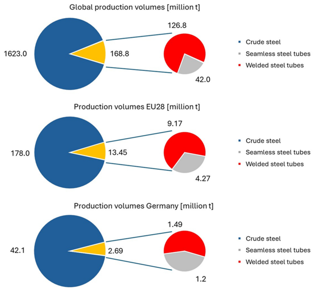
Figure 1. Classification of steel and pipe production by region and pipe production process [1,2].

Inductive longitudinal seam welding has been used industrially since the 1950s [5]. In the production of HFI-welded pipes, the starting material is continuously fed in coil form. The strip material is roll-formed into pipe bodies in an arrangement of several roll sets. Most tubing lines are flexible, with multiple sizes of tube produced on each line in a semi-continuous manner. Oftentimes, several coils of steel are welded together during a long continuous run of tubing, which may be coiled or cut to length prior to shipping depending upon product requirements.

The energy for the joining process is supplied by an inductor carrying an alternating current, which in turn induces an eddy current in the pipe cross-section. Some of the current flows along the strip edges, heating these areas through resistance heating. An upsetting roller arrangement compresses the heated strip edges in the area of the weld point, thus welding them into a closed cross-section. Contaminants such as oxides are transported from the weld seam into the weld bead [6] and often removed in-line with a deburring tool. The process thus corresponds to a resistance pressure welding process. Key advantages include high productivity due to the continuous production sequence with achievable welding speeds of up to 300 m/min [7], the good weldability of many materials, the contactless and low-wear energy supply, and the elimination of welding consumables [8]. The schematic structure of the overall process can be seen in Figure 2,where the dashed box indicates the key region of the high-frequency induction (HFI) welding process.

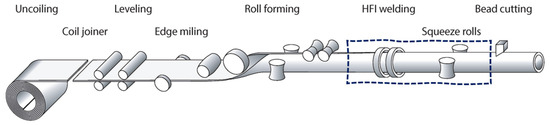
Figure 2. Schematic structure of a pipe production line for the production of HFI-welded pipes [9].

In HFI Welding, currents are induced in the tube from the induction coil and flow around the outside of the body of the tube mirroring the shape of the induction coil. As it approaches the open profile of the tube, the current begins to diverge and flow in three different paths. The most beneficial path is to flow across the strip edges along the “V” in the direction of the weld point, so that heating of the tube can take place in these areas [10]. The second most beneficial path is to flow along the strip edges towards the incoming coil of steel which results in preheating of the steel strip and eventually returns in a distributed manner across the tube or the welding rolls depending upon the mill specifics. The third pathway is undesirable and that is to return along the internal surface of the tube, which is often considered as a leakage current due to the lower resistance across the inside of the tube body as opposed to the edges [11]. The amount of current flowing in each direction depends upon the induction coil dimensions, the location of the induction coil relative to the forming rolls, and most importantly the impeder. The main role of the impeder in HFI installations is to “impede” the current flow along the internal surface [10,11].

Leakage currents flowing along the inner surface of the tube reduce the overall process efficiency by increasing the current required around the outer tube circumference, which in turn requires higher induction coil currents. Additional coil currents mean that additional kVAR’s (kilovolt-ampere reactive) are required from the capacitors, increasing the losses in the matching components. To minimize or prevent leakage current, impeders are used to increase the magnetic resistance (impedance) on the inside of the tube. By increasing the magnetic impedance inside the tube, the impeder suppresses leakage current and promotes current concentration along the strip edges, thereby improving heating efficiency and weld quality [3,12,13].

In most industrial applications, ferrite-based impeders perform this role reliably and cost-effectively, which explains their widespread use across the tube welding industry. However, certain demanding conditions reveal the practical limits of ferrite cores. At the same time, when the line speed is significantly increased or when welding small-diameter, thick-walled tubes, required magnetic loading can exceed the magnetic saturation flux density of the ferrite materials, which constrains further improvements in the system performance or even reduce the ability to maintain strong flux guidance at the weld vee. For such cases, soft magnetic composite (SMC) cores have been proposed as an alternative. SMCs are made of ferromagnetic particles insulated from one another in a polymer matrix. The proportion, shape, and distribution of the soft magnetic particles can directly influence the magnetic and electrical properties of the SMC. This makes these materials universally applicable for inductive heating in both the medium and high frequency ranges [14]. Unlike ferrites, which are brittle ceramics, SMCs are mechanically robust and can be machined into complex shapes without cracking. The magnetic properties of SMCs also prove advantageous for use as impeder core materials. Compared to ferrite impeder cores (e.g., K 2006 Bsat = 0.52 T [15]; IPH Bsat = 0.5 T [16], IPH2 Bsat = 0.51 T [16]), they possess a higher saturation flux density (e.g., Ferrotron Bsat = 1.2 T, Fluxtrol^® 100 Bsat = 1.7 T [14]), which results in SMCs exhibiting high permeability even in strong magnetic fields. These characteristics provide greater flexibility in impeder geometry and enable operation in regimes where ferrite cores exceed their magnetic limits.

At the same time, the impeder core materials used in high-frequency welding exhibit strong temperature dependence, which makes efficient cooling essential for maintaining stable magnetic performance. Ferrite and SMC impeders exhibit different temperature-dependent degradation mechanisms. In ferrites, increasing temperature reduces the saturation flux density until the Curie point is reached. In contrast, SMCs maintain relatively stable magnetic properties over a wider temperature range, but elevated temperatures reduce electrical resistivity, increase magnetic losses, and may ultimately lead to thermal failure. The critical temperature depends on the material geometry, surface coating, and cooling conditions.

In the system relevant to this study, a return-flow impeder configuration is used for cooling [17]. While required for certain products, such as galvanized tubing, this closed-loop design introduces higher flow resistance and reduces volumetric water flow compared to the same sized through-flow impeder. The cooling demand itself depends on parameters such as coolant inlet temperature, coolant pressure, welding speed, core losses, and operating frequency [18]. Reduced water flow rates lead to higher cooling-water outlet temperatures and higher ferrite core temperatures. As a result, return-flow impeders exhibit lower welding system efficiency than through-flow impeders of identical core geometry operating with the same water supply pump. Existing industrial evidence shows that significant energy savings can be achieved by replacing conventional ferrite impeders with SMC cores of higher saturation flux density, which improve magnetic efficiency and therefore reduce power consumption [18,19]. Exploring this material-based optimization pathway, specifically upgrading the impeder material from ferrite to appropriately designed SMC cores, forms a central motivation for the present work. While ferrite remains the standard solution for general applications, SMC cores may provide targeted benefits in situations where ferrite performance approaches its saturation limit.

Industrial data have further demonstrated the potential of SMC-based impeders. Field trials reported by Muyskens et al. showed that replacing ferrite cores with SMCs in tube welding systems reduced total power demand by around 40% under comparable industrial conditions [20]. Data from Fluxtrol [21] indicates that SMC impeders can achieve approximately 20–50% energy savings and significantly extend service life in their high-power tube welding applications compared with conventional designs [22]. Despite these advantages, large-scale industrial adoption of SMC impeders remains limited. The key reason is that their operational behavior differs fundamentally from ferrite, particularly in how they respond to magnetic loading and heat. These strongly coupled magnetic–thermal interactions are not adequately represented in conventional models or short-term experiments developed for ferrite systems to adequately study phenomena that take hours, days, or weeks to occur in the field. Consequently, a systematic framework supported by experimental evaluation is needed to predict SMC behavior under realistic welding conditions and to guide their reliable implementation in industrial production.

To address the limitations identified above, this study establishes a structured methodology for evaluating the performance of soft magnetic composite (SMC) impeders under realistic high-frequency induction welding conditions. The proposed methodology consists of four consecutive stages. First, high-frequency induction tube welding experiments were conducted to establish representative operating conditions for subsequent numerical simulations. The recorded process parameters and weld characteristics served as reference data for model development and initial validation. Second, a three-dimensional finite element model of the welding process was developed in ANSYS APDL 2025R1 to reproduce the main electromagnetic and thermal characteristics observed in the experiments. A three-dimensional coupled electromagnetic–thermal finite element model was then developed under a quasi-steady-state assumption. The resulting temperature distribution in the tube was then compared with the measured tube-side temperature to verify the model’s physical accuracy. Third, a simplified two-dimensional model was developed to analyze the intrinsic electromagnetic and thermal response of the impeder system. This approach was made possible by removing the steel tube with its V-shape seam from the simulation domain, leaving only the impeder and the inductor. The absence of the tube results in a rotationally symmetric geometry, which allows the problem to be represented accurately in two dimensions while significantly reducing computational cost. The configuration also makes the impeder directly accessible for experimental observation. Comparison with the full welding model confirmed that the electromagnetic environment remained comparable, and small differences in field magnitude were compensated by an equivalent scaling factor. Finally, a dedicated experimental platform corresponding to the simplified model was established. Since direct measurement of the internal impeder temperature was impractical, the cooling-water temperature was used as an experimental indicator for comparison with the numerical predictions, providing an additional assessment of the proposed methodology. Together, this method establishes a practical foundation for optimizing SMC impeder materials, cooling strategies, and process parameters in industrial high-frequency induction welding systems.

The following study presents a methodology for the off-line validation of soft magnetic composite (SMC) impeder performance in high-frequency induction welding, with Fluxtrol 50 serving as a representative example. By integrating targeted experiments with multi-stage finite element simulations, the approach enables quantitative evaluation of self-heating behavior and its dependence on magnetic loading, cooling conditions, and operating parameters. The framework also demonstrates how simulation results can be translated into practical cooling strategies to enhance thermal management. These findings provide a practical basis for optimizing impeder design and process conditions, supporting higher production efficiency and more sustainable energy use in industrial welding applications.

2. Experimental HFI Tube-Welding

2.1. Experimental Tube Welding Setup and Methods

For generating HFI welding experimental data, an experimental welding rig was developed at Chemnitz University of Technology with which pipes in a diameter range of 25 mm to 120 mm and a maximum length of 6 m can be welded. The incoming material for the experimental study must be prepared as a slotted pipe. The slotted pipe is then welded at a feed rate or velocity (v_l) of up to 40 m/min. The system includes a fin-pass roller set, which can be used to set the distance between the strip edges at a defined distance from the upsetting roller set. By varying the position of the fin-pass rollers, the vee angle α can be adjusted. The induction coil is located between the fin-pass roller set and the squeeze rolls set at a defined distance from the squeeze rolls. An SDF225 simultaneous dual-frequency generator with a maximum possible output of 150 kW (P_el,HF) in the high-frequency range (150–350 kHz) and 75 kW (P_el,MF) in the medium-frequency range (8–25 kHz) by Eldec (Dornstetten, Germany) is used to provide the electrical power. The power supply is capable of delivering either high frequency, medium frequency or both frequencies simultaneously with independent control over the power level from each frequency during operation. In addition, the impeder was positioned using a tow rod equipped with integrated cooling channels by TWTools (Balve, Germany). The impeder system bracket was designed so that the impeder position can be adjusted in three axes and the angle of the impeder relative to the workpiece can also be set. The return flow impeder, the induction coil, and the generator are all water-cooled. Furthermore, the cooling input and output volume as well as the temperature are monitored with an Endress+Hauser Picomag magnetic-inductive flow sensor (Endress+Hauser, Reinach, Swirzerland) and a type K (Ø1.0, NL100) thermocouple for calorimetric calculations.

The pair of vertical upsetting rollers can be precisely adjusted relative to each other in terms of their height. This makes it possible to minimize any strip edge misalignment that occurs. A further set of horizontal rollers is located downstream to guide the tube and the strip edges vertically. A schematic representation of the tube welding system can be found in Figure 3.

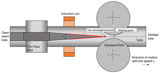
Figure 3. Schematic representation of the experimental tube welding demonstrator for manufacturing tubes with diameters ranging from 25 mm to 120 mm.

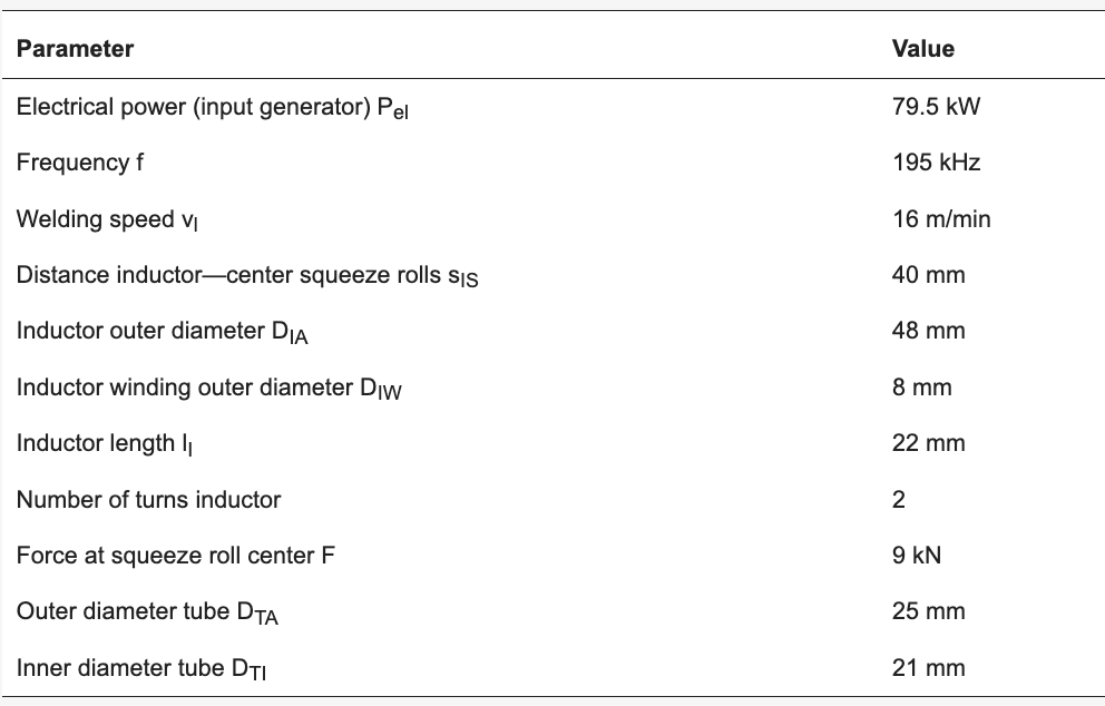
The welding system is equipped with a 120 kN Kistler 9051A force transducer (Kistler, Sindelfingen, Germany), which records the compression force on the squeeze rollers inline. This enables to measure and set the squeeze force, thereby increasing the repeatability of subsequent tests. Voltage, current, and frequency were recorded using a differential voltage probe and a Rogowski coil with an Rohde & Schwarz RTB2K-102 oscilloscope (Rohde & Schwarz, Munich, Germany). In addition, the welding speed was be determined using a speedometer of a HKS ThermoProfilScanner (Halle, Germany) monitoring system. Table 1 shows the welding parameters used in the investigations.

Table 1. Welding parameters of the reference process.

Within an experiment, the pipe is first accelerated to the welding speed. The generator is then switched on, the process conditions get constant and equivalent to continuous HFI pipe welding. In this continuous state, the process parameters are measured. The generator is switched off before the pipe is slowed down.

The workpieces used in the investigation were longitudinally welded pipes that have been cut open with a water jet at a 180° angle to the previous weld. This measure ensures that the new weld seam is free from any thermally affected zones generated during the prior fabrication of the profiles. Before the welding experiment, the workpieces must be inserted into the system. The positioning of the pipe on the fin-pass roller is particularly important, as the gap created by water jet cutting must be spread apart. The impeder is then positioned in the center of the pipe, which is made possible by the aforementioned impeder positioning system. The Fluxtrol 50 (Fluxtrol, Inc. Auburn Hills, MI, USA) impeder core material to be tested was attached to the respective impeder system.

The experimental welding system was equipped with am Optris P1M thermal camera (Optris, Berlin, Germany) for measuring a two-dimensional temperature distribution. Thereof, the maximum temperature and the temperature profile along the edges of the strip were then extracted and used for verifications with the FE simulations. To record the process thermographically, it is important to determine the emissivity, as this depends on various factors, including the surface properties of the pipe material and the view factor based upon the geometry of the region to be measured relative to the temperature measurement device. To do this, the thermal camera was positioned vertically above the pipe at an angle of 90° to the tangent of the weld seam and at a distance of 300 mm from the pipe surface. To define the process-specific emissivity, half of the pipe was painted black with thermal paint as shown in Figure 4, while the other half remains unpainted. For the coated side, an emissivity of 1.0 was assumed. The emissivity on the uncoated side was manually adjusted until the temperature values displayed corresponded to those on the coated side. The resulting emissivity value was used for the actual welding tests.

Figure 4. One-sided coated pipe for determining the emissivity during HFI welding of pipes at the laboratory.

The material used was a S235 structural carbon steel. The elemental composition was determined with Glow Discharge Optical Emission Spectroscopy (GDOES) using an Spektruma GDA750 (Spectruma Analytik GmbH, Hof, Germany). The composition can be found in Table 2, where the mean value from 9 individual measurements at different positions at one tube is given for each element.

Table 2. Element distribution for the S235 used for the tube welding trials.

2.2. Experimental Results and Discussion

Thermographic images were taken to perform a thermal analysis of the welding process. Figure 5 shows a snapshot of a weld using Fluxtrol 50 as the impeder core material. Temperature profiles were then analyzed at the vee convergence point and at defined positions upstream of the vee convergence point (v_cp) (1.5 mm, 3.0 mm, and 4.5 mm).

Figure 5. Thermographic image of a tube welding with a Fluxtrol 50 impeder core and the positions, where the temperature profiles are analyzed.

Figure 6 shows the temperature curve across the cross-section of the pipe, the assumed vee convergence point, and three defined positions in the negative process direction away from the welding point. It should be noted that the vee convergence point fluctuates during the process itself. For data analysis, we assume that the vee convergence point corresponds to the maximum temperature in the thermal camera image. Furthermore, only data within a distance of approx. 1 mm from the vee convergence point can be evaluated. One reason for this is the difficult accessibility of the optical thermography due to the narrow gap between the upsetting rolls, optical reflections on the upsetting rolls, and the roundness of the pipe, which causes the angle at which the thermal camera is positioned relative to the respective measuring point to flatten as the distance from the weld point increases.

Figure 6. Temperature curve over the distance to the edge of the band along the pipe circumference at the assumed welding point and at distances 1.5 mm, 3 mm, and 4.5 mm from the welding point in the negative process direction for the use of a Fluxtrol 50 impeder core in HFI welding at an electrical generator power of P_el = 79.5 kW and a frequency of f = 195 kHz.

In the experiment, the temperature at the edge of the strip (0.0 mm position) rises by approx. 200 K within 4.5 mm to the welding point. This relates to a rapid heating rate of 12,348 K/s considering a welding speed of v_l = 16.67 m/min. The heating rates up to 0.6 mm distance from the welding point around the tube circumference are comparable. It can also be seen that a maximum temperature of approx. 1250 °C can be measured at the vee convergence point. This value relates to a welding temperature that is approx. 279 K lower or at 84.5% of the melting temperature of the carbon steel of approx. 1528.7 °C according to a prediction after Miettinen and Howe performed with the specific alloy composition [23]. This level of welding temperature is common for press welding processes, which are carried out by combining temperature and joining pressure, whereby an increase in joining pressure enables a reduction in the thermal energy required.

For the welding test using a Fluxtrol 50 impeder core with an input power of 79.5 kW, the resulting electrical values are shown as magnitude values in Table 3. Here, both positive (Ipos, Upos) and negative (Ineg, Uneg) values are listed for current and voltage, respectively, describing the amplitude above and below the zero line.

Table 3. Results of measuring peak current, peak voltage, and frequency using Rogowski coils and voltage probes.

To measure the roundness and the diameter of the welded tubes, 3D scans using a GOM Atos Core 200 system (GOM, Braunschweig, Germany) have been performed. Afterwards, these scans were analyzed with ZEISS INSPECT Optical 3D (Version 2023) software. Figure 7 shows the geometric measurement of a welded tube. It can be seen that the loss in diameter caused by slitting the pipe and pressing out the bulge is approximately 0.15 mm.

Figure 7. Optical measurement of a welded tube showing the diameter deviations due to cutting and welding.

To evaluate the welded tubes considering the quality of the weld joint, microstructure analyses where made. Therefore, a internal defined qualitative “good” welded tube has a complete joining without any gaps. Samples with gaps where considered as not welded. The samples were ground to a fineness of 0.05 μm.

Figure 8 shows micrographs of longitudinally welded pipes using Fluxtrol 50 impeder core material. The micrographs show completely welded samples. It can be seen that there are notches in the upper and lower connection areas. In industrial installations, this area is often removed mechanically by means of a scarfing tool. This process is almost universal for external and internal beads. Its use depends on the product requirements. Furthermore, an offset can be detected. This amounts to around 10% of the sheet thickness.

Figure 8. Microscopy image of the HFI-welded tube sample using an impedance core made of Fluxtrol 50 while using the welding parameters of Table 3.

3. FEM Simulation of HFI-Welding

To complement the experimental work described above, a three-dimensional finite element (FEM) model was developed to replicate the high-frequency induction welding setup under controlled numerical conditions. The model was built using the same tube geometry, coil arrangement, impeder position, and input current level as in the experiment so that simulation results could be directly compared with measured data. Its numerical structure follows the electromagnetic–thermal coupling framework proposed by Nikanorov [24], including the solution sequence and the temperature-dependent treatment of material properties, but was adapted to reflect the specific dimensions and operating parameters of the present study. The simulation was used to calculate the electromagnetic field distribution both inside the impeder and throughout the tube–coil system. These field characteristics, which cannot be resolved directly by sensors in physical experiments, provide insight into how induced currents concentrate near the weld vee and how the impeder influences field distribution. To achieve a computationally efficient representation while preserving the dominant electromagnetic and thermal characteristics of the process, several modeling assumptions were adopted. The model focuses on the induction heating stage leading to the weld point, whereas the subsequent melting, squeeze welding, and associated mechanical deformation are beyond the scope of the present study. Tube movement is represented by an equivalent translation of the temperature field, and structural components such as clamping elements and support fixtures are omitted because of their negligible influence on the electromagnetic and thermal fields. Furthermore, the surrounding air domain is truncated sufficiently far from the region of interest, where magnetic insulation boundary conditions are applied to approximate an open boundary. These assumptions were introduced to balance computational efficiency and physical fidelity. While they may influence secondary aspects of the overall welding process, they are not expected to significantly affect the dominant electromagnetic heating behavior in the vicinity of the weld region and the impeder, which constitute the primary focus of this study. The good agreement between the numerical predictions and the corresponding experimental measurements presented in Section 6 suggests that their influence on the quantities of interest is limited under the investigated operating conditions. Model accuracy was assessed by comparing the simulated temperature evolution of the steel tube, which results from electromagnetic heating, with the measured tube-side temperature. Although small differences remain due to modeling assumptions, which will be explained in Section 6, the simulation reproduced the main temperature trends and spatial distribution observed in the experiments, confirming that the FEM model captures the essential electromagnetic behavior of the welding process.

3.1. Model Description

A three-dimensional finite element model was developed in ANSYS APDL to reproduce the high-frequency induction tube welding process with an internal impeder, as illustrated in Figure 9. The purpose of the model was to resolve the electromagnetic field distribution near the impeder and to predict the transient thermal response of the steel tube, providing complementary insight to the experimental observations reported in Section 2. A three-dimensional approach was necessary because the tube contains a V-shaped seam at the welding zone. This feature breaks rotational symmetry and prevents the use of a simplified two-dimensional axisymmetric model.

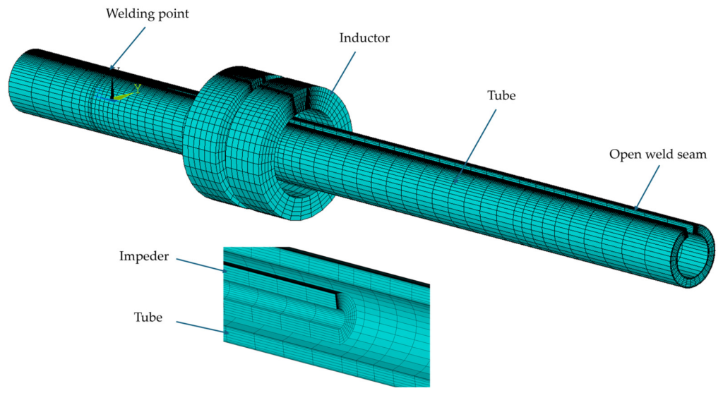
Figure 9. 3D geometry of the simulation mode.

The model geometry was constructed using the principal dimensions of the experimental setup, including the copper induction coil, the steel tube, and the soft magnetic composite (SMC) impeder. To balance accuracy and computational cost, several simplifications were introduced. The steel tube was modeled as a cylindrical shell with an open seam, represented by a V-shaped gap at the weld region to approximate the unwelded state. The surrounding air domain was included to allow correct field formation, and its outer surfaces were assigned magnetic insulation (A = 0) boundary conditions to ensure attenuation before reaching the boundaries.

The simulation was set up as an electromagnetic–thermal coupled analysis. The electromagnetic field was solved across the entire model domain in the frequency domain to obtain the magnetic flux distribution and Joule heating. The thermal field was solved only in the steel tube, because heat generation and temperature evolution in this component determine the welding outcome. Material properties such as relative permeability, thermal conductivity, specific heat, and density were taken from manufacturer data and literature [21]. A sequential solution strategy was used, where the electromagnetic results were transferred as a heat source into a transient thermal solver. Convective and radiative boundary conditions were applied to the tube surface to account for environmental heat exchange. The adopted mesh was selected based on engineering practice and was found to provide stable numerical predictions throughout the present study.

3.2. Simulation Results and Discussion

While different impeder materials were evaluated during the simulation process, the results presented here focus on a single representative case with Fluxtrol 50 SMC core to illustrate the modeling procedure and to highlight the key electromagnetic–thermal characteristics of the system. The transient temperature evolution in the steel tube was obtained by solving the thermal field using the volumetric heat source generated from the electromagnetic solution. The resulting temperature distribution is shown in Figure 10. The highest temperatures occur near the upper edge of the V-shape seam, forming a localized thermal hotspot. This behavior results from the limited skin depth at high frequencies, which confines the induced currents, and therefore the Joule heating, to the surface region of the tube beneath the induction coil. In addition, the short heating time limits thermal conduction into the tube interior. The model was designed to closely reflect the experimental configuration described in the previous section, including geometry, coil current, operating frequency, and material properties. Minor deviations are expected due to geometric simplifications and boundary assumptions, but the overall agreement supports the reliability of the coupled electromagnetic–thermal simulation approach.

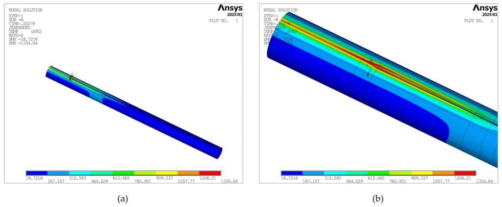
Figure 10. Temperature distribution in the steel tube: (a) Overall view; (b) Magnified view of the V-shape seam region.

To further characterize the localized heating behavior, a temperature profile was extracted along the edge of the V-shape seam (Figure 11). The temperature increases progressively toward the tip of the seam, as indicated by the curve. This trend is primarily attributed to current crowding near the joint, where the converging geometry of the seam channels the induced current more directly into the region between the strip edges. As the seam narrows, the current becomes more concentrated, generating higher local Joule heating and causing a corresponding temperature rise.

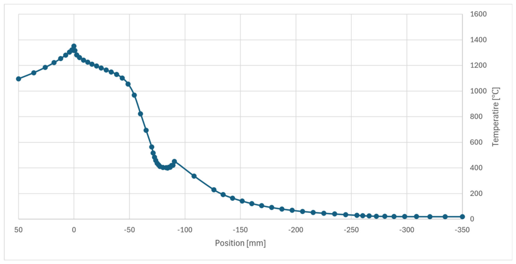
Figure 11. Temperature profile along the edge of the V-shape seam.

The simulated temperature field reflects the essential features of the thermal behavior observed in the inductive tube welding experiments described in the previous section. Because the model solves the coupled electromagnetic–thermal problem, the agreement between simulated and measured temperature distributions lends credibility to the numerical framework. Building on this comparison, the analysis next examines the electromagnetic field distribution computed within the same simulation, which provides physical insights that are not accessible through experiments alone.

The analysis focuses on magnetic flux density as a measure of how effectively the impeder material guides and shapes the magnetic field. At the same time, hysteresis loss of the impeder itself is proportional to field strength and frequency. Since frequency is fixed, to estimate losses in impeder, we need to look at how magnetic flux is distributed within the impeder during the induction welding process. Figure 12 presents the simulated magnetic flux density within the SMC impeder. Although the flux is not entirely confined within the impeder, its high permeability strongly influences the overall field distribution. A clear gradient is observed: the region directly beneath the inductor exhibits the highest flux density. This distribution confirms the impeder of this model’s function, which shapes the magnetic field near the seam correctly. To enable a meaningful comparison with the simplified 2D model presented in the following section, an additional 3D simulation was conducted including only the inductor and the impeder. The steel tube was removed to eliminate its influence on the magnetic field and to isolate the interaction between the inductor and impeder. This configuration helps clarify how the impeder responds to the applied field and provides a reference for assessing whether the 2D model captures similar field distribution under comparable conditions. The magnetic flux density distribution in this simplified setup is shown in Figure 13. The overall flux pattern resembles that of the full 3D model, with magnetic flux concentrated beneath the inductor and gradually decreasing along the impeder. While the absolute flux density is higher due to the absence of the steel tube, the spatial distribution remains consistent, differing mainly by a scaling factor. This similarity indicates that the steel tube exerts only a secondary influence on the impeder’s magnetic behavior. Therefore, for studies focused specifically on the impeder’s electromagnetic function or self-heating behavior, the tube can be omitted without significantly altering the internal field characteristics. This simplification enables more computationally efficient simulations while preserving the physical relevance of the results.

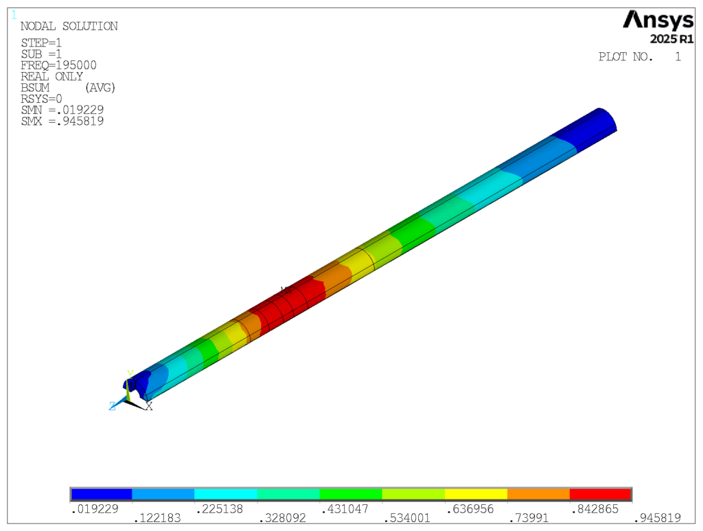
Figure 12. Magnetic flux density distribution in the SMC impeder.

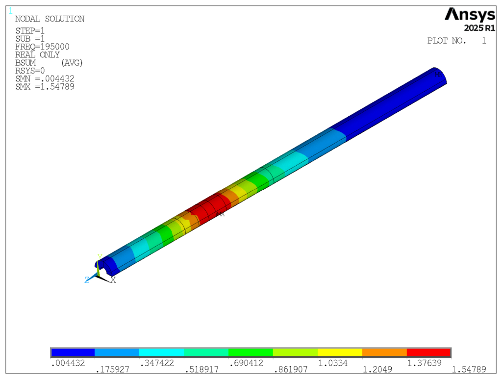
Figure 13. Magnetic flux density distribution in the SMC impeder (tube removed).

4. FEM Simulation of Long-Term Impeder Tests

To gain deeper insight into the internal behavior of the impeder beyond what can be obtained from the full welding model, a dedicated two-dimensional simulation approach was developed. The 3D model described in the previous section successfully reproduced the main electromagnetic and thermal characteristics observed in experiments, but its high computational cost and complex geometry make it less suitable for detailed studies of localized phenomena, particularly those occurring inside the impeder. These regions are also difficult to measure experimentally, which further limits the information that can be extracted from the full system model. The simplified 2D model was therefore introduced to focus specifically on the impeder’s electromagnetic and thermal response during the welding process. It is constructed to capture the dominant features of the magnetic field distribution that the impeder experiences in operation and to enable efficient simulation of field-induced heat generation and removal. While it does not replicate every detail of the 3D configuration, it preserves the essential electromagnetic environment that is necessary for analyzing the thermal behavior within the impeder. Moreover, the reduced model complexity facilitates the construction of a corresponding experimental setup, allowing the internal thermal behavior of the impeder to be investigated through a combined numerical–experimental approach over extended operating periods.

4.1. Model Description

To investigate the electromagnetic and thermal behavior of the impeder in a more targeted and computationally efficient manner, a dedicated two-dimensional finite element model was developed. This model includes only the inductor and the impeder system and is designed to capture the dominant magnetic environment experienced inside the impeder during the welding process. Its simplified geometry not only reduces computational cost while preserving the essential physical phenomena but also facilitates the construction of a corresponding physical test setup, enabling direct comparison between experimental measurements and numerical predictions.

The 2D model represents a longitudinal cross-section through the inductor–impeder assembly. Because of the geometric symmetry of the system, only half of the domain was modeled, which allows the same physical behavior to be resolved with significantly fewer elements. This reduces computational requirements without compromising simulation fidelity. The inductors were modeled as two copper blocks (orange) placed on either side of the impeder system, as shown in Figure 14. The soft magnetic composite (SMC) impeder (magenta) was mounted on a central steel rod (yellow), surrounded by a water-cooling channel (blue), and enclosed in a plastic casing (green) for mechanical support, water containment and physical protection from welding process debris. Including the water channel in the model is essential, as the impeder’s self-heating behavior is closely tied to the effectiveness of heat removal. To approximate convective cooling without explicitly solving the fluid flow, a dynamic temperature field was applied to the water layer. Instead of solving the Navier–Stokes equations, nodal temperatures were updated over time according to a predefined vertical flow velocity. The water velocity, total simulation time, and number of time steps were defined as input parameters. At each time step, nodal temperatures were updated by linear interpolation based on the assumed flow direction. This shifting temperature field effectively represents the continuous inflow of cooler water and the outflow of heated water. The inlet water temperature was fixed at 20 °C to approximate realistic operating conditions. While this approach does not capture fluid dynamics explicitly, it provides a computationally efficient method for representing the dominant effects of convective heat transfer.

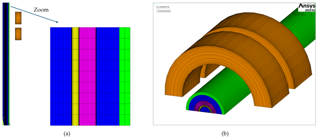
Figure 14. Geometry of the 2D simulation model: (a) Original view; (b) Symmetrical expanded view.

A key aspect of this model is the implementation of nonlinear magnetic material behavior. The μ–H curve provided by the supplier [21] was discretized into a series of data points, each representing a distinct permeability value corresponding to a specific magnetic field strength in 2 directions, as the material is anisotropic. For these models, the favorable direction is utilized for both directions based upon the way the cores were manufactured. The low permeability path is encountered only along a portion of the azimuthal direction where the flux enters and exits the core, which inherently is much larger in area than the axial direction of flow of the flux through the core, limiting its impact on the simulation results. During the simulation, the magnetic field intensity (H) was computed for each element at every time step. The local permeability (μ) was then updated element by element based on the most recent H value, ensuring that the magnetic response of the SMC material evolved dynamically with the field conditions. This iterative updating procedure captures the nonlinear magnetic characteristics of the impeder and significantly improves the physical fidelity of the simulation. The thermal conductivity (λ) of the SMC was defined as anisotropic according to supplier data [21], reflecting the directional dependence of heat transport within the composite. For the thermal analysis, heat generation within the SMC was calculated using a loss equation supplied by the manufacturer [21]. This equation accounts for both hysteresis and eddy current contributions and enables the simulation to capture field-dependent self-heating behavior under realistic operating conditions.

To avoid boundary reflections and ensure accurate field resolution, the air domain extended well beyond the inductor–impeder assembly, and magnetic insulation (A = 0) was applied on the outer surfaces to represent an open boundary. A locally refined mesh was used in the impeder region and other areas with steep field gradients to improve solution accuracy. Material properties for copper, steel, and the SMC were defined consistently with those used in the 3D model described in Section 3.1.

In cases where the impeder exhibits a non-rotationally symmetric geometry, such as the fluted designs commonly employed in industrial practice, an equivalent radius for the impeder core is defined based on an equal mass of magnetic material rather than the conventional outer and inner diameter definitions. The validity of this equivalent-mass approach was recently demonstrated by Goldstein and Muyskens, who compared five different impeder cores with two distinct cross-sections under experimental operating conditions similar to those used in the present work. Their results were evaluated against finite-element calculations based on the equivalent-mass formulation for a 10 mm equivalent hollow impeder core, as presented at Fabtech 2025. Excellent agreement was obtained between simulation and measurement, both for electrical operating parameters and for calorimetrically determined core loss at 200 kHz with maximum flux densities approaching approximately 1.2 T. These findings also justify the use of only the high-permeability direction in the two-dimensional electromagnetic analysis. The corresponding results are illustrated in Figure 15. For such geometries, a supplementary two-dimensional radial-cut model taken through the region of maximum flux density is additionally proposed for evaluating the local temperature distribution within the impeder core. In this model, appropriate surface heat-transfer coefficients are imposed to confirm that the resulting core temperatures remain within acceptable operating limits [25].

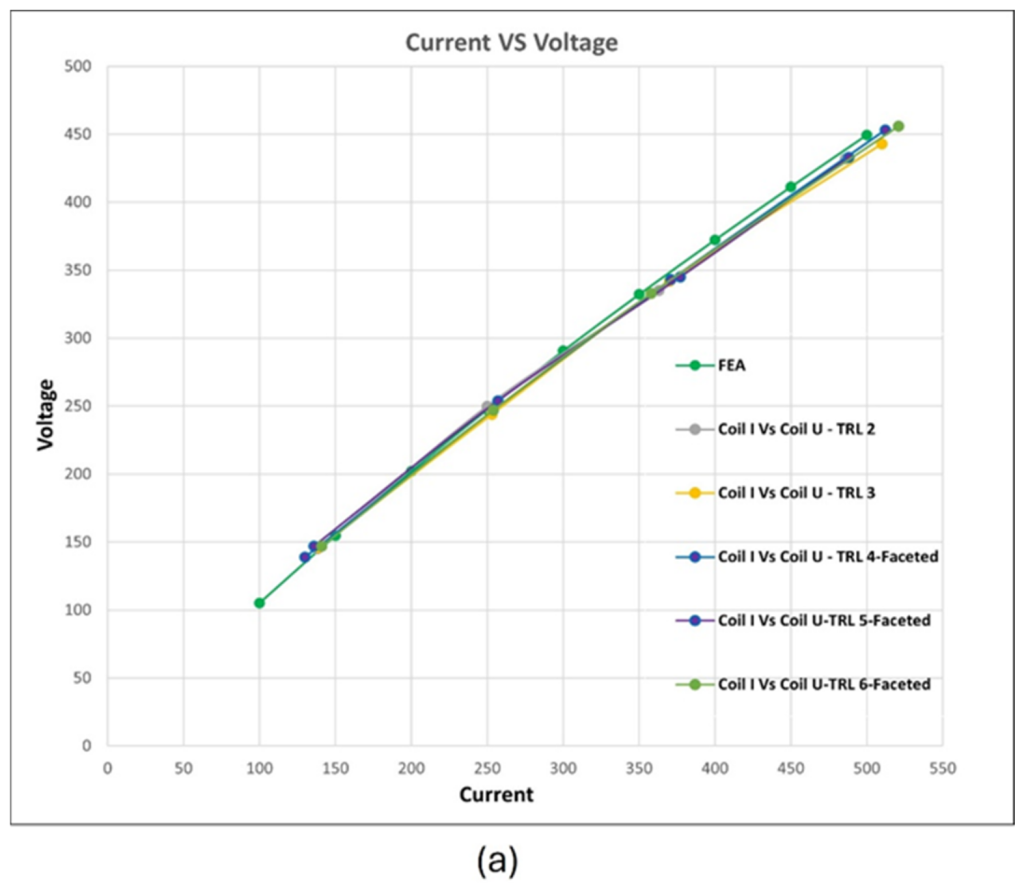
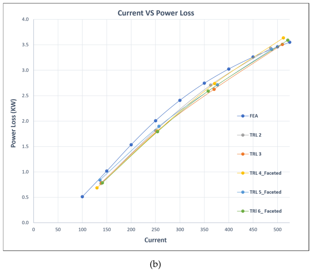
Figure 15. Comparison between finite-element predictions and experimental measurements for a 10 mm equivalent hollow impeder core at 200 kHz: (a) voltage-current characteristics; (b) core power loss-current characteristics.

4.2. Comparison with 3D Welding Model

Before the thermal analyses were carried out, the electromagnetic performance was first compared with the corresponding 3D impeder-only model, which serves as the reference solution for the model reduction. This comparison was necessary to verify that removing the steel tube and simplifying the domain geometry did not significantly alter the key magnetic characteristics within the impeder system. Establishing a consistent electromagnetic response was considered an essential prerequisite for using the 2D model to investigate internal thermal behavior in the subsequent analyses. Figure 16 provides a direct visual comparison of the magnetic flux distribution in the impeder region for both the 2D and 3D impeder-only models. Although the dimensions of the inductor and impeder differ slightly—mainly to simplify the construction of a corresponding experimental setup—the spatial patterns of the magnetic field remain closely aligned. Both models show a pronounced gradient from the region beneath the inductor to the rest of the impeder, with the magnetic flux density reaching its maximum directly under the inductors and gradually decreasing along the impeder length.

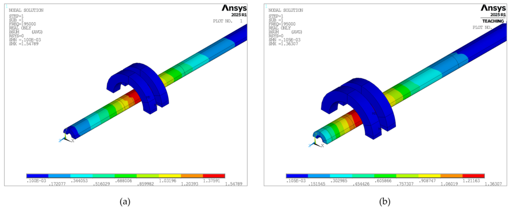
Figure 16. Magnetic flux density comparison between the 2D model and the 3D impeder-only model: (a) B-distribution of impeder in 2D model (expanded view); (b) B-distribution of impeder in the 3D impeder-only model.

While the 2D model cannot replicate the complete three-dimensional field behavior, the strong visual similarity of the field patterns confirms that it captures the dominant features required for thermal analysis. In particular, the gradient of magnetic flux from the under-inductor region toward the impeder ends is preserved, as is the overall confinement of flux within the SMC material. This distribution is critical because the spatial pattern of magnetic excitation governs the regions and intensity of heat deposition within the impeder. The fact that the flux remains largely confined within the impeder further demonstrates that the SMC material continues to serve its guiding function even under the 2D approximation. For a more meaningful visual comparison, the input current in the 2D simulation was adjusted so that the resulting flux density magnitude closely matched that of the 3D reference model. This scaling compensates for differences in geometry and boundary conditions while maintaining comparable electromagnetic conditions across both models. The scaling factor is determined by matching the overall magnetic flux density distribution of the reduced 2D model to that of the corresponding 3D reference model under the same operating conditions. It should therefore be regarded as a configuration-specific calibration parameter rather than a universal correction coefficient. Since its value depends on the particular geometry, operating conditions, and material properties of the investigated system, it is recalibrated whenever the reference configuration changes. Consequently, the proposed methodology is generally applicable, whereas the numerical value of the scaling factor is system dependent. Although the match is not exact, the overall field shape, magnitude, and direction show sufficient consistency. The resulting agreement in the magnetic field distribution supports the use of the 2D model for analyzing field-driven heating behavior, while substantially reducing the computational effort compared with the full 3D model.

Overall, the 2D model offers a reliable and computationally efficient framework for investigating the impeder’s internal thermal behavior. Compared with the corresponding 3D model, the computational time was reduced from approximately 8 h to 1.5 h under the same computational condition, making the proposed approach well suited for extensive parametric investigations. It preserves the essential electromagnetic features responsible for heat generation while enabling faster simulations and easier integration with experimental measurements. With its capability to isolate the impeder’s response to magnetic excitation, the 2D model serves as a powerful tool for targeted studies that would be difficult or prohibitively expensive to conduct using a full 3D simulation. This foundation also sets the stage for the subsequent thermal analysis, which examines self-heating behavior and the effects of cooling strategies in greater detail.

4.3. Temperature Distribution in the Impeder

With the electromagnetic field distribution in the 2D model established, a transient thermal simulation was conducted to investigate the temperature distribution within the SMC impeder. The volumetric heat source was derived from the magnetic flux density obtained from the steady-state electromagnetic solution, using a supplier-provided loss equation that accounts for both hysteresis and eddy current losses. This enabled a spatially resolved calculation of heat generation inside the impeder and the subsequent temperature evolution during the welding process.

The initial temperature of the domain was set to 20 °C. Because explicit fluid flow was not modeled, the cooling water region was represented through an equivalent thermal boundary treatment. A thin interfacial layer was introduced only at the surfaces in contact with the cooling water to approximate the net heat extraction effect without solving the fluid domain. This layer was assigned temperature-dependent thermal properties derived from empirical correlations relevant to induction cooling conditions [26]. As a result, it provides a realistic thermal coupling between the impeder system and the surrounding coolant while maintaining the computational efficiency of a fully solid model. Beyond this layer, a dynamic temperature field was applied to the water region to emulate the effect of continuous flow, allowing nodal temperatures to be updated according to a prescribed vertical velocity and time step.

Figure 17 shows the simulated temperature field within the impeder after a representative heating period. The highest temperatures are concentrated in the region directly beneath the inductor, consistent with the area of maximum magnetic flux density. The temperature decreases gradually along the impeder length, forming a distinct axial gradient. This distribution arises from the combined effects of gradient in magnetic flux density and resultant power density in the core. Even with water cooling surrounding the system, the inner region directly beneath the inductor remains the dominant hotspot because it is located deep within the SMC body. Magnetic power density is relatively uniform in the cross-section, but the temperature is highest as this location is farther away from the convective cooling. The thermal conductivity of the material determines heat dissipation from this region to the cooled outer surface.

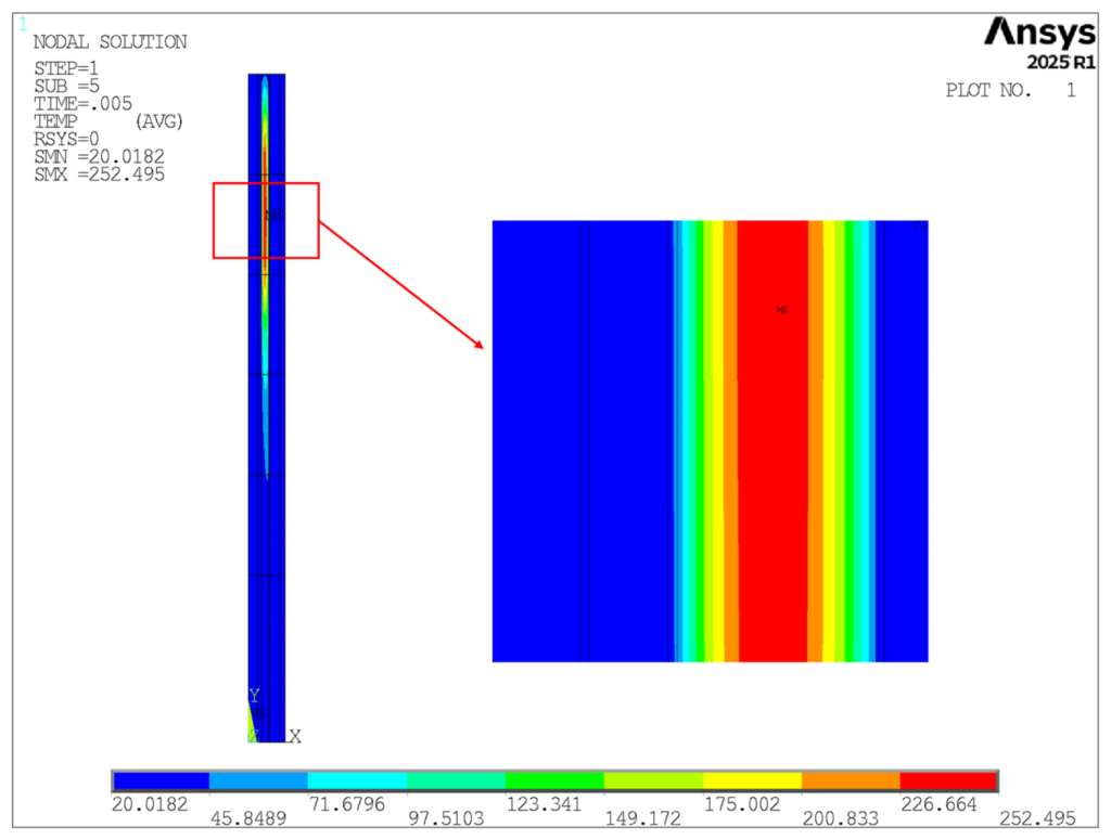
Figure 17. Steady state temperature distribution within the impeder system.

The temperature variation in the cooling water layer is related to the internal thermal dynamics of the impeder. With the inlet temperature maintained at 20 °C, the simulated outlet water temperature increases to about 45 °C under steady-state conditions at the exit (Figure 18). This temperature rise represents the cumulative heat transferred from the impeder surface to the coolant, and the predicted trend shows good consistency with what is expected under similar operating conditions. Since the internal temperature of the impeder is not directly accessible, the change in water temperature provides a practical and physically meaningful indicator of the overall total losses in the system and a way to compare the results to experiments and verify that overall coolant flow is sufficient to remove the losses. It also provides insights into internal core material temperatures, which will be extremely difficult to measure during testing and can identify conditions for potential local core failure or in the case of ferrites, core performance decline.

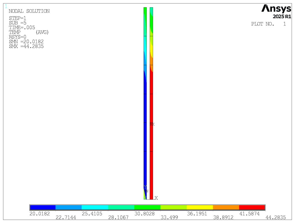
Figure 18. Temperature distribution of the cooling water.

In summary, the transient thermal simulation demonstrates how the spatial distribution of magnetic flux governs the formation of temperature gradients inside the impeder. The region directly beneath the inductors remains the thermally most critical zone, as the localized power density gradients are a stronger influence than the cooling fluid temperature increasein the SMC material. Although explicit fluid convection was not modeled, the adopted equivalent thermal boundary treatment successfully reproduces the expected cooling trend and the rise in outlet water temperature. This confirms that the 2D model captures not only the internal heating mechanisms but also the measurable thermal response at the boundaries. The model achieves a balance between computational efficiency and physical fidelity, providing the accuracy required to assess impeder performance under realistic welding conditions. Furthermore, its ability to reproduce both localized temperature concentrations and overall heat transfer behavior makes it a valuable tool for further investigation and design. The predicted outlet water temperature also offers a practical and accessible benchmark for future experiments, enabling direct comparison between experimental measurements and numerical predictions. Taken together, these findings establish a reliable foundation for design analysis and performance optimization of impeder components in industrial high-frequency induction welding systems.

5. Experimental Long-Term Impeder Tests

Experimental Long-Term Test Setup and Methods

To provide experimental data for comparison with the FE simulation under continuous operating conditions, a calorimetric test system for long-term impeder measurements was developed. The basic structure of the system consists of aluminum profiles, with a metal tray at the bottom to protect against escaping cooling water. The test chamber is further protected in all directions by 3 mm thick acrylic glass so that adequate protection can be ensured in the event of the impeder system overheating and arcing. In addition, the system has an access point for exhaust gas extraction to remove any toxic gases that may occur due to thermal decomposition of polymers present. The inductor and the impeder are fed in from the side through an access point. Both tools have an integrated return cooling system and are therefore water-cooled throughout the entire test process. The type and positioning of the inductor are usually equivalent to the pipe welding configuration. The generator used is an eldec induction HFG 50 generator with a usable electrical power up to 50 kW and a frequency range from 80 kHz to 450 kHz. The inductor used is the same as for tube welding (Table 1). The measuring instruments for recording the electrical parameters (oscilloscope, voltage probes) are also the same. Since there is no open tube in the test setup, lower power values than for pipe welding are required to replicate a flux density comparable to the inside of a tube during HFI welding. Figure 19 shows the continuous test facility, including the system components it contains.

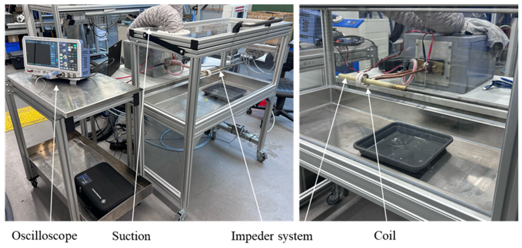
Figure 19. Long-term test facility at Chemnitz University of Technology for measuring the heating of the cooling water in the impeder under continuous operating conditions and drawing conclusions about the heating of the impeder core, including the possibility of predicting failure due to overheating.

The tests were carried out according to the procedure described in Figure 20 left. First, the impeder core to be tested was installed in the impeder system and then in the test rig, ensuring that it is aligned centrally with the inductor. After the cooling medium has been supplied, the generator was started with the corresponding target power. The temperature curve was recorded inline and displayed live as shown in Figure 20 on the right side. For all tests, the measured flow rate was in the range of v = 0.6…0.7 L/min.

Figure 20. Experimentally recorded temperature curve during a series of endurance tests using Fluxtrol 50, with a test duration of t = 20 min, a frequency f = 180 kHz and a generator output of Pe1 = 1.5 kW (left), as well as the schedule for an endurance test (right).

It can be seen that the outlet temperature initially rises steeply and then stabilizes at a plateau. It is assumed that the impeder at the plateau level operates in steady-state condition. When the generator is switched off, the outlet temperature of the cooling medium also decreases sharply until it returns to the inlet temperature. This means the thermal mass is minimal. The inlet temperature and flow rate remain constant throughout the entire process.

During the endurance tests, the flow rate, input, and output temperatures are recorded using an Endress + Hauser Picomag flow-meter as well as a mantle thermocouple type K, ø 1.0, NL100. Figure 21 shows the relationship between the temperature increase in the cooling water and the variation in generator power P_el.

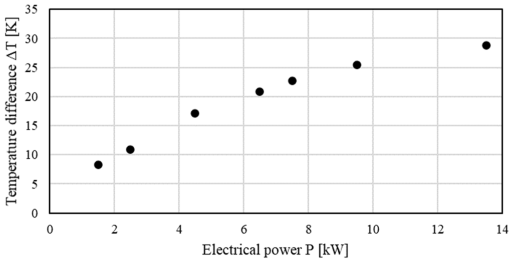
Figure 21. Temperature difference ΔT of the inlet and outlet temperature of the cooling medium across generator input power P_el using a Fluxtrol 50 impeder core on the endurance test rig.

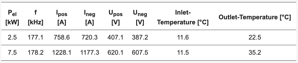
At the same time, electrical parameters are measured using a Rogowski coil and voltage probes. This allows the frequency, current, and voltage to be measured during the test. The measurement results are shown in Table 4.

Table 4. Measurements taken with an oscilloscope during continuous testing on the Fluxtrol 50 Impeder at generator power ratings of P_el,1 = 2.5 kW and P_el,2 = 7.5 kW.

To evaluate the endurance tests, both the input and output temperatures of the cooling medium at the inlet and outlet of the impeder system were recorded. The resulting temperature delta can then be used to determine the amount of heat loss that occurs in the impeder core and is dissipated via the cooling medium, taking into account the heat capacity c, density ρ, the output and the input temperature (Toutput and Tinput) and flow rate v present in the process, using the equation below. This is an indicator of the impeder core heating and possible overheating of the magnetic field concentrator.

𝑄˙=𝑣×𝜌×𝑐×(𝑇𝑜𝑢𝑡𝑝𝑢𝑡−𝑇𝑖𝑛𝑝𝑢𝑡)

To determine the relationship between the electrical power fed into the system via the generator as a setting parameter and the resulting amount of heat loss, a series of tests was first carried out using the impeder core material Fluxtrol 50. An output temperature of the cooling medium of T = 50 °C was set as the maximum value for this set of trials, and the electrical power was gradually increased until this value was reached. The resulting findings can be found in Figure 22. A nearly linear relationship between input power and the resulting rate of heat change can be observed over the range of power levels studied. It is also important to note that the impeder losses are only about 10% of the generator electrical power. The main losses in the system are in the induction coil and power supplying circuitry, even without the most resistive component in a tube welding system, the open tube, not being present. This further reinforces the concept that even though the core losses are much higher for the SMC cores, they are only a small fraction of the overall power in the system and the resultant benefits from their application far outweigh the additional core loss.

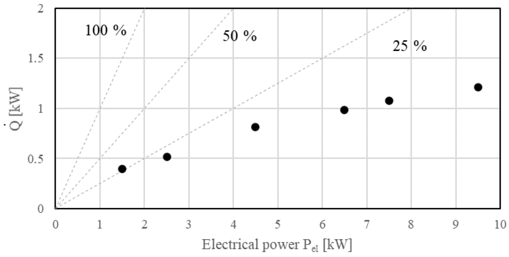
Figure 22. Rate of heat change, which is absorbed by the cooling medium during the continuous test and provides information about the temperature increase in the impeder core, above the input generator power, using the example of a Fluxtrol 50 impeder at a frequency range of f = 177…179 kHz.

Further tests were carried out with a higher generator output. However, these led to thermal failure of the Fluxtrol 50 impeder core, which is shown in Figure 23. During the stabilization phase (2), heavy smoke developed in the test rig. This resulted in the failure of the protective cover and the escape of coolant through the cracks that had formed in the protective cover. A generator output power of P_el = 13.5 kW was used for this. It can be seen that the impeder core shows significant black discoloration, especially in the area below the inductor. Other than that, the impeder core itself was geometrical unchanged. This shows that it is possible with the test rig to deliberately and controllably bring the impeder system, especially the protection tube, to its respective power limit. The highest measured temperature of the outgoing cooling water was T = 40.0 °C.

Figure 23. Thermally damaged Fluxtrol 50 impeder after a continuous test at a generator output of P_el = 13.5 kW.

–

By testing the impeders in a continuous test rig, it is possible to examine them under continuous process conditions with regard to the existing magnetic field and the resulting losses in the impeder core. However, effects affecting the pipe are neglected. These include, for example, the heating of the pipe, which influences the induced magnetic field due to temperature-dependent changes in electrical conductivity. Furthermore, damage to the impedance device caused by welding spatter cannot be investigated on the existing test rig. In reality, however, this often leads to the failure of magnetic field concentrators. Another problem is the inability to measure the temperature directly at the impeder core. Since this is a reflux impeder system with an impeder protective cover, optical thermography cannot be used.

6. Experimental Evaluation of the Numerical Model

The methodology proposed in this work is based on a combined use of experimental measurements and numerical simulations, where two experimental setups are coupled with their corresponding simulation models to derive key performance quantities. Since the predictive capability of the proposed methodology depends on the agreement between experimental observations and numerical predictions, a systematic comparison of both is required.

In this section, the proposed methodology is assessed through a systematic comparison of experimental measurements and numerical predictions obtained under matched operating conditions. The comparison aims to evaluate how well the proposed methodology reproduces the experimentally observed behavior and captures the dominant physical phenomena.

The welding experiment is first used to evaluate the predictive capability of the corresponding numerical model by comparing the measured and simulated temperature distributions along the weld seam. In the experiment, the temperature profile was obtained using an infrared camera. Due to the measurement range limitation of the device, only the temperature values within the valid detection range were considered for evaluation. In contrast, the numerical model provides the complete temperature distribution along the seam without such constraints. To ensure a meaningful comparison, the model inputs were defined based on experimentally measured parameters (shown in Section 1), including the operating frequency, input current, and the geometrical dimensions of the relevant components, so that the simulation conditions are consistent with the experimental setup.

Figure 24 presents the comparison between the measured and simulated temperature profiles. A high level of agreement is observed within the valid measurement range, indicating that the model is capable of accurately capturing the thermal behavior in the welding zone. The simulation well reproduces the overall shape and peak characteristics of the temperature distribution. A slight deviation can be observed in the region downstream of the welding point, where the simulated temperature decreases more gradually than the experimental results. This difference is likely attributed to the cooling effect induced by the contact between the rollers and the steel tube in the experiment. Such contact-related heat transfer is not included in the numerical model, which leads to a slower predicted temperature decay.

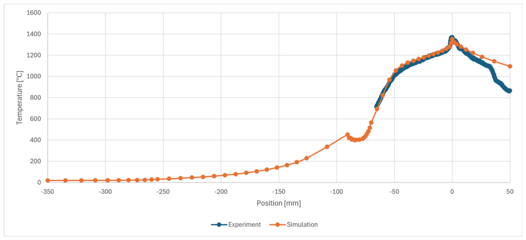
Figure 24. Agreement between experimental and simulated seam temperature.

Overall, the good agreement between the experimental and numerical temperature distributions demonstrates that the model provides a reliable representation of the thermal behavior during the welding process.

The second experimental comparison follows a different workflow. The numerical model is first established, and the corresponding geometrical and operating parameters are then provided to Chemnitz University of Technology for the construction of the experimental setup. Due to the limited accessibility of the impeder during operation, direct measurements of its internal temperature and electromagnetic behavior are not feasible. Therefore, the model is assessed indirectly by comparing the predicted and measured cooling water temperatures, which provide an experimentally accessible indicator of the overall thermal performance of the impeder.

In the general simulation presented in the previous sections, an inlet cooling water temperature of 20 °C was adopted as a representative operating condition. For the present experimental validation, however, the numerical model was updated using the experimentally measured inlet water temperature of 11.5 °C to ensure consistent boundary conditions between the simulation and the experiment. Figure 25 presents the simulated cooling water temperatures at an input current of 1200 A. The predicted outlet water temperature reaches 32.6 °C, while the corresponding experimental measurements reported by Chemnitz University of Technology show an inlet temperature of 11.5 °C and an outlet temperature of 35.2 °C under comparable operating conditions.

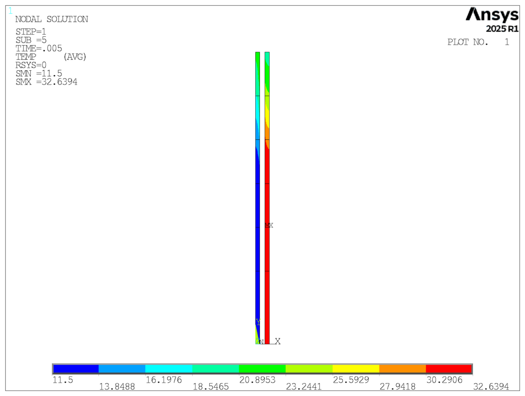
Figure 25. Temperature distribution of the cooling water.

The comparison demonstrates good agreement between the numerical prediction and the experimental measurements. The remaining discrepancy can be attributed to uncertainties associated with both the experimental measurements and the numerical model. Based on the temperature rise in the cooling water, the deviation between the simulation and experiment is approximately 12%. Considering that the outlet water temperature represents the cumulative effect of heat generation within the impeder, heat conduction through the surrounding components, and convective heat transfer to the cooling water, a certain level of discrepancy is expected. In addition, unavoidable uncertainties associated with infrared temperature measurement, emissivity estimation, effective convective heat transfer coefficients, cooling water flow conditions, material properties, and other experimental operating conditions may further contribute to the observed deviation. Since the cooling water temperature serves as an indirect validation quantity rather than a direct measurement of the impeder temperature, the obtained agreement is considered satisfactory for validating the proposed electromagnetic–thermal modelling methodology. Overall, the comparison confirms that the numerical model is capable of predicting the overall thermal behavior of the impeder with reasonable accuracy.

Taken together, the two experimental comparisons demonstrate the capability of the proposed methodology to reproduce the key thermal responses observed under the investigated operating conditions. The first comparison shows good agreement between the predicted and measured temperature distributions along the weld seam under consistent operating conditions. The second comparison further demonstrates that the proposed methodology can reliably predict the overall thermal response of the impeder, as reflected by the cooling water temperature under comparable operating conditions. Despite the indirect nature of the second validation, the consistent agreement between the numerical predictions and the experimental observations in both comparisons supports the applicability of the proposed experimental–numerical methodology for analysing the thermal behaviour of SMC impeders. The validated methodology is therefore considered suitable for the subsequent parametric investigations presented in this work.

7. Conclusions

This study introduced a structured approach for examining the electromagnetic and thermal behavior of soft magnetic composite (SMC) impeders under realistic high-frequency induction welding conditions. By integrating welding experiments with a sequence of finite element models, the work established a reliable basis for evaluating how SMC cores respond to the coupled field and temperature environment characteristic of high-speed welding processes.

The welding experiments provided the operating parameters and reference measurements needed to anchor the numerical analysis. Using these data, a three-dimensional model was developed to reproduce the field distribution and temperature evolution near the weld region. Comparisons with measured tube-side temperatures showed that the simulations captured the governing thermal trends, supporting the suitability of the modeling assumptions for representing the welding environment. To focus on the intrinsic behavior of the impeder, a simplified two-dimensional model was constructed. This configuration retained the essential electromagnetic characteristics of the system while substantially reducing computational cost. The corresponding laboratory setup enabled direct observation of the cooling water temperature, which served as a practical indicator of the impeder’s thermal response. The comparison between measurements and simulations demonstrated consistent trends and reasonable agreement, confirming the physical relevance of the modeling approach. Overall, the results provide a solid foundation for understanding and improving the performance of SMC impeders in industrial tube welding. The study shows that combining targeted experiments with physics-based modeling can support material evaluation, guide impeder design, and contribute to better thermal stability and energy efficiency during high-frequency induction welding.

Looking forward, several avenues for further development of the impeder system emerge from this work. Although the methodology was demonstrated using Fluxtrol 50 as a representative SMC material, it is not limited to this specific material. Its application to other SMC materials requires only the corresponding material properties, while the resulting performance and any calibration parameters remain material-dependent. Improvements may be achieved by optimizing the internal cooling configuration to promote more effective heat removal, by adjusting the core geometry to balance magnetic guidance and thermal loading, or by exploring SMC formulations with improved thermal and magnetic stability. Future work may also incorporate Navier–Stokes-based computational fluid dynamics to resolve the detailed coolant flow and local heat transfer within the impeder. Such an approach could complement the present electromagnetic–thermal methodology by providing a more detailed representation of the cooling process under complex operating conditions.

Author Contributions

Conceptualization, Y.Z., I.N., D.G., M.K. and R.C.G.; methodology, Y.Z. and I.N.; software, Y.Z.; validation, Y.Z. and D.G.; formal analysis, Y.Z.; resources, R.C.G.; writing—original draft preparation, Y.Z. and D.G.; writing—review and editing, Y.Z., D.G., R.C.G. and M.K.; supervision, E.B. and M.K.; project administration, E.B.; funding acquisition, E.B. All authors have read and agreed to the published version of the manuscript.

Funding

This research was funded by the ZIM program of the German Federal Ministry for Economic Affairs and Climate Action, project number KK5385602KX2.

Data Availability Statement

The data supporting the findings of this study are available from the corresponding author upon reasonable request.

Acknowledgments

The authors would like to thank Alexander Nikanorov for valuable technical support in the development of the numerical model. We also thank Till Clausmeyer for his helpful comments on earlier versions of this manuscript. We also appreciate the valuable discussions with D. Scott MacKenzie that contributed to the development of this work. During the preparation of this manuscript, the authors used ChatGPT (OpenAI, GPT-5.3) for language refinement and editing. The authors have reviewed and edited the output and take full responsibility for the content of this publication.

Conflicts of Interest

Author Robert C. Goldstein was employed by the company Fluxtrol, Inc., Auburn Hills, USA. The remaining authors declare that the research was conducted in the absence of any commercial or financial relationships that could be construed as a potential conflict of interest. The funders had no role in the design of the study; in the collection, analyses, or interpretation of data; in the writing of the manuscript; or in the decision to publish the results.

Abbreviations

The following abbreviations are used in this manuscript:

SMC	Soft Magnetic Composite
HFI	High-frequency induction

References

1. World Steel Association. Steel Statistical Yearbook 2018; World Steel Association: Brussels, Belgium; Beijing, China, 2018. [Google Scholar]
   
2. Wirtschaftsvereinigung Stahlrohre e.V. Jahresbericht 2017; Wirtschaftsvereinigung Stahlrohre e.V.: Düsseldorf, Germany, 2018; Available online: http://www.wv-stahlrohre.de/jahresbericht.html (accessed on 5 May 2022).
   
3. Kim, H.J.; Youn, S.K. Three dimensional analysis of high frequency induction welding of steel pipes with impeder. J. Manuf. Sci. Eng. 2008, 130, 031005. [Google Scholar] [CrossRef]
   
4. Kang, C.; Shi, C.; Liu, Z.; Liu, Z.; Jiang, X.; Chen, S.; Ma, C. Research on the optimization of welding parameters in high-frequency induction welding pipeline. J. Manuf. Process. 2020, 59, 772–790. [Google Scholar] [CrossRef]
   
5. Wallace, R.C.; Stanton, R.C. Induction welding. U.S. Patent US2763756A, 18 September 1956. [Google Scholar]
   
6. Inoue, T.; Suzuki, M.; Okabe, T.; Matsui, Y. Development of advanced electric resistance welding (ERW) linepipe “mighty Seam^TM” with high quality weld seam suitable for extra-low temperature services. JFE Tech. Rep. 2013, 18, 18–22. [Google Scholar]
   
7. O’Brien, A.; Guzman, C. Welding handbook. In Welding Processes, Part 2; American Welding Society: Miami, FL, USA, 2007; Volume 3. [Google Scholar]
   
8. Nacke, B.; Baake, E. Induction Heating: Heating, Hardening, Annealing, Brazing, Welding; Vulkan-Verlag: Essen, Germany, 2016. [Google Scholar]
   
9. Egger, C.; Lüchinger, M.; Schreiner, M.; Tillmann, W. Numerical Simulation of Tube Manufacturing Consisting of Roll Forming and High-Frequency Induction Welding. Materials 2022, 15, 1270. [Google Scholar] [CrossRef] [PubMed]
   
10. Milićević, M.; Radaković, Z. Quality improvement of steel pipes produced by seam welding with new magneto-dielectric impeder. Mater. Trans. 2006, 47, 1464–1468. [Google Scholar] [CrossRef]
    
11. S. W. AG. HF-Welding Impeder-Technologie; S. W. AG: Frankfurt am Main, Germany, 2017. [Google Scholar]
    
12. Milicevic, M.S.; Milicevic, V.M. Impeder for HF inductive welding of steel tubes. IEE Proc. Sci. Meas. Technol. 2002, 149, 113–116. [Google Scholar] [CrossRef]
    
13. Milićević, M.S.; Nejković, V.M. Implementation of Optimal Hf Welding Procedure of Steel Pipes for High-Quality and Energy-Efficient Welds. Proc. Rom. Acad. Ser. A Math. Phys. Tech. Sci. Inf. Sci. 2024, 25, 55–64. [Google Scholar] [CrossRef]
    
14. Polytron Kunststofftechnik GmbH. Ferrotron & Fluxtrol—Focus on Induction. Available online: https://www.polytron-gmbh.de/frontend/media/files/polytron-werkstoffbroschuere-ferroton-fluxtrol.pdfx (accessed on 8 July 2026).
    
15. Kaschke Components GmbH. Material K 2006 Für Impederkerne; Kaschke Components GmbH: Göttingen, Germany, 2011. [Google Scholar]
    
16. T.S.E. GmbH Tube Scarfing Equipment. Ferrite Cores (Impeder Cores). Available online: www.tube-scarfing.com (accessed on 8 July 2026).
    
17. DeSaw, F.A. Induction Welding Impeder Apparatus with Fluid Cooling. US4443677A, 17 April 1984. [Google Scholar]
18. Return Flow Impeders Manufacturer, Supplier, Exporter- Latest Price. Available online: https://www.mungipaelectricals.in/return-flow-impeders-6849608.html (accessed on 5 May 2022).
    
19. Return Flow Impeders. Available online: https://www.kentcorporation.com/consumables/impeders/return-flow-impeders/ (accessed on 5 May 2022).
    
20. Muyskens, S.M.; Eddir, T.I.; Goldstein, R.C. Improving induction tube welding system performance using soft magnetic composites. COMPEL Int. J. Comput. Math. Electr. Electron. Eng. 2020, 39, 185–191. [Google Scholar] [CrossRef]
    
21. Fluxtrol | Fluxtrol 50 Soft Magnetic Composite for Induction Heating. Available online: https://fluxtrol.com/fluxtrol-50 (accessed on 8 July 2026).
    
22. Muyskens, S.; Goldstein, R. Characterization of Soft Magnetic Composite Impeders. Available online: https://www.fluxtrol.com/characterization-of-soft-magnetic-composite-impeders/ (accessed on 8 July 2026).
    
23. Miettinen, J.; Howe, A.A. Estimation of liquidus temperatures for steels using thermodynamic approach. Ironmak. Steelmak. 2000, 27, 212–227. [Google Scholar] [CrossRef]
    
24. Nikanorov, A.; Baake, E.; Neumeyer, J. Numerical Simulation and Investigation of High Frequency Tube Welding Process. Appl. Mech. Mater. 2014, 698, 245–250. [Google Scholar] [CrossRef]
    
25. Goldstein, R.; Muyskens, S. Improving HF Tube Welding System Performance Using SMC Impeder Cores. Available online: https://www.fluxtrol.com/improving-hf-tube-welding-system-performance-using-smc-impeder-cores/ (accessed on 8 July 2026).
    
26. Golovin, G.F.; Zimin, N.V. Tekhnologiya Termicheskoy Obrabotki Metallov S Primeneniem Induktsionnogo Nagreva (Technology of Heat Treatment of Metals Using Induction Heating), 5th ed.; Mashinostroenie: Leningrad, Russia, 1990. (In Russian) [Google Scholar]

Disclaimer/Publisher’s Note: The statements, opinions and data contained in all publications are solely those of the individual author(s) and contributor(s) and not of MDPI and/or the editor(s). MDPI and/or the editor(s) disclaim responsibility for any injury to people or property resulting from any ideas, methods, instructions or products referred to in the content.

© 2026 by the authors. Licensee MDPI, Basel, Switzerland. This article is an open access article distributed under the terms and conditions of the Creative Commons Attribution (CC BY) license.